Original Paper by: Leonard Berrada, Andrew Zisserman, M. Pawan Kumar
High Level Overview
- Cross entropy (CE) loss is the theoretically optimal loss for top-k classification in the limit of infinite data, but given noisy and limited data it is possible to design a loss function that improves on CE.
- Properties of such a loss function include:
- Smooth
- Non-sparse gradients
- It is possible to rewrite the multi-class SVM loss in a way such that it can be smoothed with a temperature parameter. Furthermore its calculation can be made tractable using polynomial algebra and divide-conquer techniques.
- The results confirm that in scenarios with limited and noisy data, smooth multi-class SVM loss outperforms CE significantly
Introduction
CE loss functions are theoretically ideal given infinite data for top-k classification tasks. However it is prone to overfit in the case of limited noisy data. Therefore we can introduce a multi-class SVM loss to maximise the margin between the correct top-k predictions and the incorrect ones. However these loss functions have sparse gradients and consequently do not perform well with deep neural networks. To alleviate this sparsity, the paper introduces a smooth loss function with an adjustable temperature.
Related Work
-
Previous work applying top-k loss functions concentrates on shallow/linear models.
-
Previous work on smoothing SVM functions has either been on binary tasks, or has approached it differently (i.e., using Moreau-Yosida regularisation).
Top-K SVM
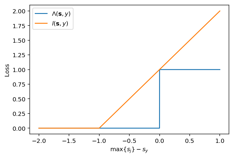
Following the notation in the paper, we observe that a simple prediction and loss over the the top-1 class prediction given a score vector $\mathbf{s}$ and label $y$ would be:
\[\begin{equation} P(\mathbf{s}) \in \arg\max \mathbf{s} \end{equation}\] \[\begin{equation} \Lambda(\mathbf{s},y) \triangleq \Bbb{1}(y \neq P(\mathbf{s})) = \Bbb{1}(\underset{j\in \mathcal{Y}}{\max} s_j > s_y) \label{eq:top-1-loss} \end{equation}\]This loss however is non-continuous, and clearly non-differentiable. To ameliorate this there exists the SVM hinge loss to act as an upper bound:
\[\begin{equation} l(\mathbf{s},y) = \max\left\{ \underset{j\in \mathcal{Y} \setminus y}{\max} \{ s_j + 1 \} - s_y, 0 \right\} \end{equation}\]To illustrate the difference (and upper-boundedness) clearly, observe the following comparison:
There is then the natural extension to the top-k case:
\[\begin{equation} P_k(\mathbf{s}) \in \left\{ \bar{y} \in \mathcal{Y}^{(k)}: \forall i \in \{ 1,\dots,k \}, s_{\bar{y}_i} \geq s_{[k]} \right\} \end{equation}\]i.e., give the k-tuple for which all entries are greater than or equal to the $k$-th largest score.
\[\begin{equation} \Lambda_k(\mathbf{s},y) \triangleq \Bbb{1}(y \neq P_k(\mathbf{s})) = \Bbb{1}( s_{[k]} > s_y) \label{eq:top-k-loss} \end{equation}\]i.e., check if $y$ is in the prediction k-tuple (where $s_{[k]}$ is the $k$-th highest score).
We then write the corresponding surrogate:
\[\begin{equation} l_k(\mathbf{s},y) = \max\left\{ \underset{j\in \mathcal{Y} \setminus y}{\max} (\mathbf{s}_{\setminus y} + \mathbf{1})_{[k]} - s_y, 0 \right\}. \label{eq:surrogate-topk} \end{equation}\]We observe that this is now weakly differentiable, but not smooth. This results in sparse gradients that reduce the efficacy of neural nets trained with this loss function, even when testing on training data (i.e., it’s not a generalisation/regularisation problem).
The appendix shows a way to reformulate \ref{eq:surrogate-topk} to make it amenable to smoothing:
\[\begin{equation} l_k(\mathbf{s},y) = \underset{\bar{\mathbf{y}} \in \mathcal{Y}^{(k)}}{\max}\left\{\Delta_{k}( \bar{\mathbf{y}}, y) + \sum_{j \in \bar{\mathbf{y}}} s_j \right\} - \underset{\bar{\mathbf{y}} \in \mathcal{Y}^{(k)}_y}{\max}\left\{\sum_{j \in \bar{\mathbf{y}}} s_j \right\} \label{eq:reform-topk} \end{equation}\]which is then naturally smoothed to
\[\begin{equation} L_{k,\tau}(\mathbf{s},y) = \tau\log\left[\sum_{\bar{\mathbf{y}} \in \mathcal{Y}^{(k)}} \exp \left( \frac{1}{\tau} \left(\Delta_{k}( \bar{\mathbf{y}}, y) + \frac{1}{k} \sum_{j \in \bar{\mathbf{y}}} s_j \right) \right) \right] - \tau \log \left[ \sum_{\bar{\mathbf{y}} \in \mathcal{Y}^{(k)}_y} \exp \left( \frac{1}{k\tau}\sum_{j \in \bar{\mathbf{y}}} s_j \right)\right]. \label{eq:smooth-topk} \end{equation}\]This loss has the following interesting properties:
- For $\tau > 0$, it is infinitely differentiable and non-sparse.
- As $\tau \rightarrow 0^+$, we observe $L_{k,\tau}(\mathbf{s},y) \rightarrow l_k(\mathbf{s},y)$ in a point-wise manner.
- $L_{k,\tau}(\mathbf{s},y)$ is an upper bound on $l_k(\mathbf{s},y)$ iff $k = 1$, but is actually an UB, up to a scaling factor, on $\Lambda_k$ for all $k$.
The paper also notes that in the case the margin $\alpha \rightarrow 0^+$ and $\tau = 1$, CE is retreieved.
Computational Challenges and Efficient Algorithms
This is more concerned with algorithms rather than ML, so we will skip this section for now.
Results
In summary, CE outperforms Smooth top-k loss in the case of full CIFAR-100 data. However, when noise is added to the labelling (such that the top-k isn’t affected), smooth top-k loss greatly outperforms CE, and this increases with additional noise. Interestingly, in top-1 classification, the smooth top-k with $k=5$ greatly outperforms CE when noise is introduced, despite the fact that the task at hand is not a surrogate to the true loss.
The loss is also tested on ImageNet data, and it is observed that apart from when 100% of the data is available, smooth top-k loss outperforms CE.
Conclusion
- By smoothing the top-k SVM surrogate loss, we achieve non-sparse gradients and therefore improved performance on deep neural nets.
- In the case of noisy/limited data, the resultant smooth top-k loss outperforms CE, as the latter will tend to overfit, despite being theoretically justified in the limit of infinite data.
- Perhaps the idea of smoothing can be carried over into other surrogate losses, as this may help generalisation.